This page is Part 3 in a series of pages explaining the science of good measurement. The previous page gave an introduction to uncertainty evaluation and introduced the concept of an uncertainty budget. Concepts such as uncertainty, traceability and proving conformance were introduced in Part 1. In this page I give a full explanation of how to calculate an uncertainty budget for a length measurement using vernier callipers.
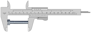
The example of the measurement of a bolt using a set of callipers is used on this page. A number of sources of uncertainty are considered; Calibration (xcal) error in mm; Resolution (xres) error in mm; Cosine Error (xcos) angular misalignment; Temperature (xT) error in degrees C; Repeatability (xrep) error in mm. The measurement result (y) is a function of these input quantities as well as the actual length of the measurand (Y). Unlike in previous examples the input quantities have different functional relationships with the measurement result. The functional relationship between these quantities can be written.
Also unlike in previous examples the input quantities have different probability distributions, and different units. This all results in a more complex uncertainty budget. The simple uncertainty budget used in the previous lecture assumed a simple y=x1+x2… xn functional relationship, that all the input uncertainties had the same units and that they were all normally distributed.
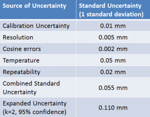
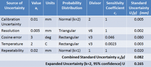
This page explains step by step how a full uncertainty budget is calculated. For each input uncertainty the units of measurement and probability distribution must first be stated. A divisor is used to account for the way that different probability distributions contribute different amounts to the combined uncertainty. A sensitivity coefficient is used to adjust the input value for different units of measurement and for the way in which it contributes to the combined uncertainty.
Adding Sources with different Probability Distributions to the Uncertainty Budget
First we will look in more detail at the different types of probability distribution which input uncertainties may have and the divisors used for these.
Uncertainties which are determined through repeated measurements are called Type A, they are generally assumed to follow a normal distribution. Calibration uncertainty is also assumed to be a normal distribution and is simply divided by the coverage factor for the given level of confidence. For example if a 95% confidence level calibration uncertainty is given then it is divided by the coverage factor 2.
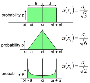
Uncertainties obtained from other means such as estimates or specifications are called Type B, these may follow a rectangular distribution especially where hard limits are given for an input quantity or little other information is available. A rectangular distribution means that there is zero probability of the value lying outside of the limits and an equal probability of having any value within the limits. The limits of a distribution are called the semi-range limits (a), two rectangular distributions with limits of +/-a combine to give a triangular distribution of +/-2a. U-shaped distributions are sometimes encountered in electronics. More than two distributions of any shape will combine to give an approximately normal distribution according to the central limit theorem. The standard uncertainty which is contributed to the combined uncertainty can be obtained by dividing the semi-range limits by a divisor.
Sensitivity Coefficients
Sensitivity coefficients allow us to add sources together which have different units of measurement and/or different functional relationships
Where the relationship between the input quantities and the measurement result does not have a simple functional relationship of the form y=x1+x2… xn it is necessary to define sensitivity coefficients describing how the inputs contribute to the combined uncertainty. In the GUM this is given in the form of a partial differential equation, the partial differentials simply describe the rate at which the measurement result will change if one of the input quantities changes. Since we generally know the approximate value of the measurement result we can simply calculate a sensitivity coefficient ci in place of these terms which gives the ratio for change in the measurement result per unit change in the input. Simplifying the equations also means that we can multiply the uncertainty in the input by the sensitivity coefficient before squaring. For the mathematically minded this is shown below, otherwise this is most easily understood with some examples.
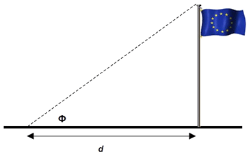
Consider the measurement of the height of a flagpole by measuring the horizontal distance and the angle of inclination. The height (H) is given by
H = d tanΦ
If d is 10 m +/-0.1 m and Φ is 27° +/-0.1° then the height is nominally 5.095 m
The sensitivity of the height measurement to a change in d can be found by calculating H using the extreme values of d. So if d=10.1 then h=5.146 or if d=9.9, h=5.044
Comparing with the nominal values, the change in H divided by the change in d gives the sensitivity coefficient for d:-
cd=ΔH/Δd=0.5095
Similarly the sensitivity to a change in the angle Φ can also be calculated using the extreme values of Φ
If Φ=27.1 then H=5.117 and Δh/ΔΦ =0.2200
If Φ=26.9 then H=5.073 and Δh/ΔΦ =0.2196
Since in this case Φ is involved in a trigonometric function the sensitivity coefficient does not have a constant value, taking the average of the extreme values is however a reasonable approximation for uncertainty estimation.
cΦ ≈ 0.22
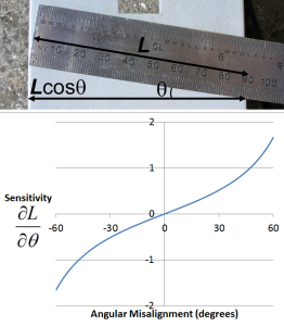
Cosine error is commonly encountered in dimensional measurement due to angular misalignment. In this case the sensitivity coefficient is zero for the change in unit length per change in unit angle varies greatly depending on the size of the angular error. It is therefore normal practice to use the extreme values. For example for a nominal length of 100 mm, an angular error of +/- 3° could result in errors in the measured length of 100(1-cos 3°) = 0.137 mm. Dividing this maximum length error by the maximum angular error of 3° gives sensitivity coefficient of 0.046 mm/degree.
Another common example of the use of a sensitivity coefficient is for thermal expansion. In this case the change in length (ΔL) is equal to the change in temperature (ΔT) multiplied by the nominal length (L) and the coefficient of thermal expansion for the material (α). This can be rearranged to give the sensitivity of the change in length to a change in temperature (ΔL/ ΔT).
For example for a 100 mm aluminium bolt the coefficient of thermal expansion is 23×10-6 K-1 therefore the sensitivity coefficient is 0.0023 mm/°C
Calculating Standard Uncertainties
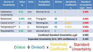
Having determined the value, probability distribution, divisor and sensitivity coefficient for each source of uncertainty these can now be used to calculate a standard uncertainty for each source. Each source of uncertainty’s value is divided by its divisor and multiplied by its sensitivity coefficient to give its standard uncertainty. Due to the use of the sensitivity coefficients the standard uncertainties now give the uncertainty in the measurement result (y) due to each source of uncertainty rather than the input quantities (xi), there are therefore denoted ui(y).
Calculating the Combined Standard Uncertainty
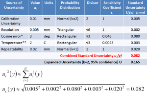
Having calculated the standard uncertainties the combined standard uncertainty can now be calculated. For the mathematically inclined, since the sensitivity coefficients have been used to obtain the standard uncertainties in terms of the uncertainty in the measurement result the partial derivatives require no further consideration. The combined uncertainty therefore becomes simply the square root of the sum of each standard uncertainty squared (RSS). The simplification of the GUM equation is shown here although it is not necessary to understand this in order to calculate the uncertainty budget.
The calculation of the combined standard uncertainty is easily understood by considering our example uncertainty budget. Each standard uncertainty is squared, the results are added up and the square root of the sum is taken. In other words the combined standard uncertainty is the root sum square (RSS) of the individual standard uncertainties.
Using a Coverage Factor to Calculate the Expanded Uncertainty
Since the combined uncertainty has a normal distribution we have only 68% confidence that the true value lies within +/- the combined standard uncertainty uc(y) of the measurement result. It is therefore standard practice to multiply the combined standard uncertainty by a coverage factor (k) to give the Expanded Uncertainty (U). We have now covered all the steps involved in creating a full uncertainty budget for a measurement process or calibration.
Using the uncertainty budget to prove conformance or non-conformance with a specification
Once the uncertainty has been determined for a measurement process it can then be used to establish whether a measurement proves conformance or non-conformance with a specification. There are cases where measurements are not conclusive in which case a statement such as this should be used.
“The result is below/above the specification limit by a margin less than the measurement uncertainty; it is therefore not possible to state compliance/non-compliance based on the stated level of confidence. However the result indicates that compliance/non-compliance is more probable than non-compliance/compliance with the specification limit.”
Now that you understand the correct scientific way to evaluate uncertainty of measurement lets consider another way. Measurement Systems Analysis (MSA) and Gage R&R have many practical uses but they also have some